Introduction
This project is attempt to assign ICD9 codes autonomously to clinical notes in eletronic medical records through machine learning models.
Data
The MIMIC-III dataset was used to train all models. Since this was a multilabel text classification task, a fair amount of preprocessing was necessary. Clinical notes were embedded (converted from text to a dense vector representation) with word2vec embeddings pretraiend on Google News and BERT embeddings pretrained on the MIMIC-III dataset. Results using the BERT embeddings, though, have not yet been obtained. ICD9 codes were grouped with the clinical notes on the hadm_id column in MIMIC-III. This resulted in a varying number of ICD9 codes being associated with each clinical note (hence the multilabel classification task).
Exploratory visualizations of the dataset can be found in this section.
Models
The baseline models trained for this task were a logistic regression, a random forest, and a multilayer perceptron. The word2vec embeddings were element-wise averaged across all words in a given note to obtain a document representation.
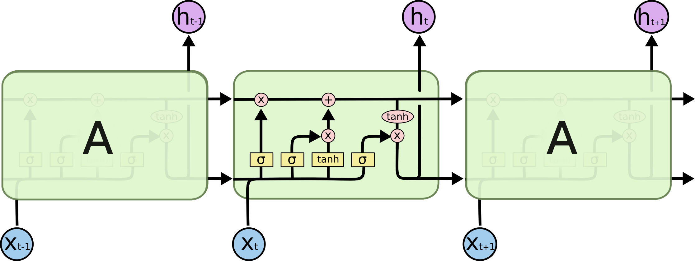 A long short-term memory model was also trained using PyTorch in an attempt to leverage sequential relationships between words in clinical notes.
Results from the models that were trained can be found here.
Note: LSTM image obtained from http://colah.github.io/posts/2015-08-Understanding-LSTMs/
Read Data
import pandas as pd
import numpy as np
import functools as ft
import itertools as it
import os
from typing import List, Set, Dict, Tuple
from utils import get_conn, query_aws, PROJ_DIR, TREE, V_CODE
import tqdm
import spacy
from itertools import chain
from collections import Counter
import torch
import math
import re
pd.set_option('display.max_colwidth', -1)
nlp = spacy.load("en_core_web_sm")
# read in list of all notes
notes_df = query_aws("select text from mimiciii.noteevents limit 50000")
notes = notes_df["text"].tolist()
# set data locations
datadir = os.path.join(PROJ_DIR, "data", "preprocessed")
imagedir = os.path.join(PROJ_DIR, "images")
modeldir = os.path.join(PROJ_DIR, "data", "models")

# load all processed data (with embeddings excluded)
df = pd.read_pickle(os.path.join(datadir, "visdata.pd"))

# load test data
test_df = pd.read_pickle(os.path.join(datadir, "test.pd"))
Y_test = test_df["roots"].tolist()
class_names = pd.read_csv(os.path.join(datadir, "class_names.csv"),
                          header=None, squeeze=True).tolist()
# add root names to df
get_codes = lambda dummies: [class_names[i] for i, dum in enumerate(dummies) if dum]
df["root_names"] = df["roots"].apply(get_codes)
Exploratory Visualizations
from scripts.visdata import summary_table, note_lengths, icd_summary
import matplotlib.pyplot as plt
import seaborn as sns
from wordcloud import WordCloud
Summary Tables
# load summary table data
summ_df = summary_table(query_aws)
row_order = ["Patients", "Admissions", "ICD9 Codes", "Deaths"]
col_order = ["Totals", "Male", "Female", "Private", "Medicare", "Medicaid", "Government", "Self Pay"]
summ_df = summ_df.loc[row_order, col_order]
summ_df
ICD9 Summary
Due to the granularity of ICD9 codes, only the top level of codes in the ICD9 hierarchy were used for classification. They are summarized below.
all_roots = list(it.chain.from_iterable(df["root_names"].tolist()))
icd_table = icd_summary(all_roots, TREE)
icd_table
Categories
Clinical notes are binned (exclusively) into several different cateogories.
query = "select category, count(row_id) from mimiciii.noteevents group by category;"
ccounts_df = query_aws(query)
ccounts_df.columns = ["Category", "Count"]
ccounts_df = ccounts_df.sort_values("Count", ascending=False)
cat_fp = os.path.join(imagedir, "categories.png")
ax = sns.barplot(x="Category", y="Count", data=ccounts_df)
ax.set_title("Counts by Category")
plt.setp(ax.get_xticklabels(), ha="right", rotation=45)
plt.tight_layout()
plt.savefig(cat_fp)
plt.show()

Distributions
icd_lens = [len(r) for r in df["root_names"].tolist()]
note_lens = notes_df["text"].apply(lambda s: len(re.findall(r'\w+', s)))
note_lens_mid = lens[lens.between(lens.quantile(.1), lens.quantile(.9))]
ax = sns.distplot(icd_lens)
ax.set(xlabel="Number of Top Level ICD Codes",
       title="Distribution of Top Level ICD Codes per Note")
plt.savefig(os.path.join(imagedir, "num_icd_codes.png"))
plt.show()

ax = sns.distplot(note_lens_mid)
ax.set_title("Distribution of Number of Words in a Note")
ax.set_xlabel("Word Count")
plt.savefig(os.path.join(imagedir, "word_counts.png"))

plt.show()


ICD Codes by Insurance
# read data
query = """
SELECT admissions.hadm_id AS adm_id, count(diagnoses_icd.icd9_code) AS icd, array_agg(admissions.insurance)[1] AS insurance
FROM mimiciii.admissions AS admissions
JOIN mimiciii.diagnoses_icd AS diagnoses_icd
ON admissions.hadm_id = diagnoses_icd.hadm_id
GROUP BY admissions.hadm_id;
"""
insur_icd_df = query_aws(query)
ax = sns.boxplot(x="insurance", y="icd", data=insur_icd_df)
ax.set(xlabel="Number of ICD9 Codes",
       ylabel="Insurance Type",
       title="Number of ICD Codes per Admission by Insurance Type")
plt.savefig(os.path.join(imagedir, "insurance.png"))
plt.show()

Word Cloud
wordcloud = WordCloud(max_font_size=50, max_words=100, background_color="white").generate(notes[15])
plt.figure()
plt.imshow(wordcloud, interpolation="bilinear")
plt.axis("off")
plt.savefig(os.path.join(imagedir, "wordcloud.png"))
plt.show()

Embedding Comparisons
from gensim.models import KeyedVectors
from transformers import AutoTokenizer, AutoModel
# load word2vec
w2v_fp = os.path.join(PROJ_DIR, "data", "embeddings",
                      "GoogleNews-vectors-negative300.bin")
word2vec = KeyedVectors.load_word2vec_format(w2v_fp, binary=True)

# load bert
bert = AutoModel.from_pretrained("emilyalsentzer/Bio_ClinicalBERT")
bert.eval()
tokenizer = AutoTokenizer.from_pretrained("emilyalsentzer/Bio_ClinicalBERT")
from torch.nn.utils.rnn import pad_sequence
T = [torch.tensor(tokenizer.encode(n, add_special_tokens=True)) for n in notes[0:31]]
pX = pad_sequence(T)
e = bert(pX)
Results
import torch
import torch.nn as nn
from torch.nn.utils.rnn import pad_sequence, pack_padded_sequence
from transformers import BertModel
Load Classifiers
import joblib
from scripts.models import Clf, Lstm
from sklearn.base import BaseEstimator
from sklearn.metrics import (f1_score, precision_score, recall_score,
                             classification_report)
from scripts.evaluation import ml_accuracy, probs_to_preds
def predict(model, X: List[List[int]], threshold: float = 0.5) -> np.ndarray:
    """Give predictions for the given data."""
    probs = model(X)
    pos = torch.where(probs < threshold, probs, torch.ones(*probs.shape))
    neg = torch.where(pos > threshold, pos, torch.zeros(*probs.shape))
    preds = neg.long().numpy()
    return preds

def predict_proba(model, X: List[List[int]]) -> np.ndarray:
    """Get probabilities for the given data."""
    return model(X).detach().numpy()
# load base classifiers
clf_fns = ["LogisticRegression.sk", "RandomForest.sk", "MLP.sk"]
clfs = [Clf(joblib.load(os.path.join(modeldir, fn)), fn.split(".")[0])
        for fn in clf_fns]
# get predictionss for each clf
for clf in clfs:
    clf.set_preds(test_df["d2v"].tolist())
    clf.set_probs(test_df["d2v"].tolist())
# load lstms
lstm_w2v_fn = "Lstm_w2v1.pt"
lstm_w2v = Lstm(torch.tensor(word2vec.vectors))
lstm_w2v.load_state_dict(torch.load(os.path.join(modeldir, lstm_w2v_fn)))
lstm_w2v.eval()
preds = []
for x in tqdm.tqdm(test_df["w2v_idx"].tolist()):
    preds.append(predict(lstm_w2v, [x]))
probs = []
for x in tqdm.tqdm(test_df["w2v_idx"].tolist()):
    probs.append(predict_proba(lstm_w2v, [x]))
clf = Clf(lstm_w2v, "Lstm_w2v")
clf.preds = preds
clf.probs = probs
clfs.append(clf)
Performance Results
# get performance data
f1s = [f1_score(Y_test, clf.preds, average="weighted", zero_division=1) for clf in clfs]
precs = [precision_score(Y_test, clf.preds, average="weighted", zero_division=1) for clf in clfs]
recs = [recall_score(Y_test, clf.preds, average="weighted", zero_division=1) for clf in clfs]
metrics = f1s + precs + recs
met_labels = ["F1 Score"] * len(clfs)+ ["Precision"] * len(clfs) + ["Recall"] * len(clfs)
clf_names = [clf.name for clf in clfs] * 3
ax = sns.barplot(x=clf_names, y=metrics, hue=met_labels)
ax.set_ylim([0, 1])
ax.set(title="Model Performance Comparison")
plt.savefig("data/images/model_comparison.png")
plt.show()

Classification Reports
class_reports = {clf.name: classification_report(Y_test, clf.preds, target_names=class_names,
                                             zero_division=1, output_dict=True)
                 for clf in clfs}
crep_dfs = {name: pd.DataFrame(crep).T for name, crep in class_reports.items()}
crep_df = pd.concat(crep_dfs, axis=1)
crep_df
Probability Distributions
fig, axs = plt.subplots(1, len(clfs), sharey="all", sharex="all")
for ax, clf in zip(axs, clfs):
    ax.hist(np.array(clf.probs).flatten())
    ax.set(title=clf.name)
fig.set_size_inches(10, 5)
fig.suptitle("Predicted Probability Distributions")
plt.savefig("data/images/prob_dists.png")
plt.show()

Precision/Recall Curves
def pr_curve(clf_name, probs, y_true, thresholds):
    """
    Generate precision/recall curve data for a given classifier.

    Implementation is custom because sklearn doesn't
    support multilabel classification for pr curve.
    """
    precs = []
    recs = []
    for thresh in tqdm.tqdm(thresholds):
        preds = probs_to_preds(probs, thresh)
        precs.append(precision_score(y_true, preds, average="weighted", zero_division=1))
        recs.append(recall_score(y_true, preds, average="weighted", zero_division=1))
    data = {"Classifier": [clf_name] * len(thresholds),
            "Precision": precs,
            "Recall": recs,
            "Threshold": thresholds}
    return pd.DataFrame(data)
# extract precision/recall data across thresholds
thresholds = np.linspace(0, 1, 10)
pr_dfs = [pr_curve(clf.name, clf.probs, Y_test, thresholds) for clf in clfs]
pr_df = pd.concat(pr_dfs)
# plot precision recall curve for each classifier
ax = sns.lineplot(x="Recall", y="Precision", hue="Classifier", data=pr_df)
ax.set_ylim([0.5, 1])
ax.set_xlim([0, 1])
ax.set(title="Precision Recall Curve")
plt.savefig("data/images/prec_rec.png")
plt.show()
